ML Model Blue Bike Demand Prediction
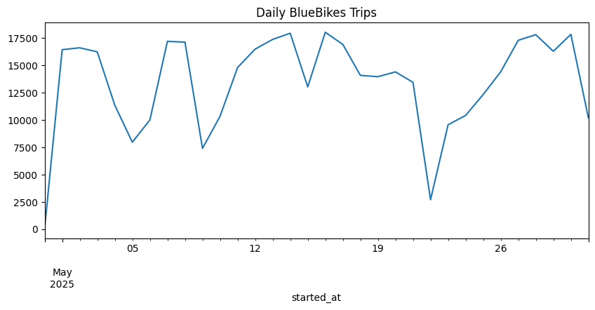
I set out to forecast hourly demand for Blue Bikes using real trip data (start/end station, timestamp, rideable type). My goal was to build a model that could support operations planning—knowing in advance how many bikes will be needed at each hour of the day. I was first interested in this idea when I saw a Blue Bike station that was new and realized I didn't know how they decided they had enough bikes to meet demand.
1. Data Preparation
-
Feature Extraction
Loaded the raw CSV of every trip, parsed the start time into separate
date,hour,dayofweek,is_weekend, andis_holidaycolumns. Filtered down to justdate,hour, the calendar flags, andtotal_tripsper hour via a grouped aggregation. -
Train/Test Split
Sorted chronologically and used the last 6 days as a hold-out test set; the prior data (all earlier dates) became my training set.
2. Baseline: Linear Regression
My first attempt was a simple linear regression on the four calendar features (hour, dayofweek, is_weekend, is_holiday):
from sklearn.linear_model import LinearRegression

                    lr = LinearRegression()
                    lr.fit(X_train, y_train)
                    y_pred = lr.predict(X_test)
Result: RMSE ≈ 475.15, MAE ≈ 370.90/em>.
Insight: The straight-line fit couldn’t capture the sharp morning/evening peaks or weekend vs. weekday shifts.
3. Model Exploration & Leaderboard
To find a better algorithm, I looped through all scikit-learn regressors using a 3-fold TimeSeriesSplit, evaluating MAE and RMSE for each:
from sklearn.utils import all_estimators
        from sklearn.model_selection import TimeSeriesSplit, cross_validate

                    # Loop through regressors, collect CV MAE/RMSE into a DataFrame…
This produced a “leaderboard” (top 10 shown):
| Model | MAE | RMSE |
|---|---|---|
| RadiusNeighborsRegressor | 208.21 | 334.59 |
| KNeighborsRegressor | 215.33 | 346.70 |
| GaussianProcessRegressor | 230.50 | 384.38 |
| BaggingRegressor | 232.29 | 378.11 |
| RandomForestRegressor | 232.30 | 381.48 |
| ExtraTreesRegressor | 234.21 | 387.18 |
| DecisionTreeRegressor | 236.30 | 390.14 |
| ExtraTreeRegressor | 236.96 | 390.35 |
| HistGradientBoostingRegressor | 237.86 | 363.27 |
| GradientBoostingRegressor | 240.59 | 367.05 |
Table 1. Top 10 scikit-learn regressors by cross-validated MAE.
Winner: RadiusNeighborsRegressor (MAE ≈ 208) captured local patterns by averaging demand from “nearby” hours in feature-space.
4. Hyperparameter Tuning
I wrapped the radius-neighbors model in a Pipeline (with StandardScaler) and ran a GridSearchCV over:
radius: [0.5, 1, 2, 5, 10]weights: ['uniform','distance']metric: ['euclidean','manhattan']leaf_size: [20, 30, 40]
from sklearn.neighbors import RadiusNeighborsRegressor
                    from sklearn.model_selection import GridSearchCV, TimeSeriesSplit
                    from sklearn.pipeline import Pipeline
                    from sklearn.preprocessing import StandardScaler

                    pipe = Pipeline([
                    ("scale", StandardScaler()),
                    ("rnr", RadiusNeighborsRegressor())
                    ])
                    param_grid = {
                    "rnr__radius":      [0.5,1,2,5,10],
                    "rnr__weights":     ["uniform","distance"],
                    "rnr__metric":      ["euclidean","manhattan"],
                    "rnr__leaf_size":   [20,30,40]
                    }
                    grid = GridSearchCV(
                    estimator=pipe,
                    param_grid=param_grid,
                    cv=TimeSeriesSplit(5),
                    scoring="neg_mean_absolute_error",
                    n_jobs=-1,
                    verbose=2
                    )
                    grid.fit(X_train, y_train)
Best CV MAE: MAE ≈ 184.75868055555554
Best Params:
{
                    "radius": 5.0,
                    "weights": "distance",
                    "metric": "manhattan",
                    "leaf_size": 20
                    }
5. Final Evaluation
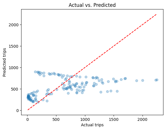
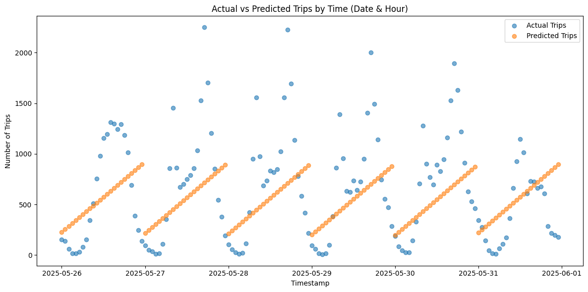
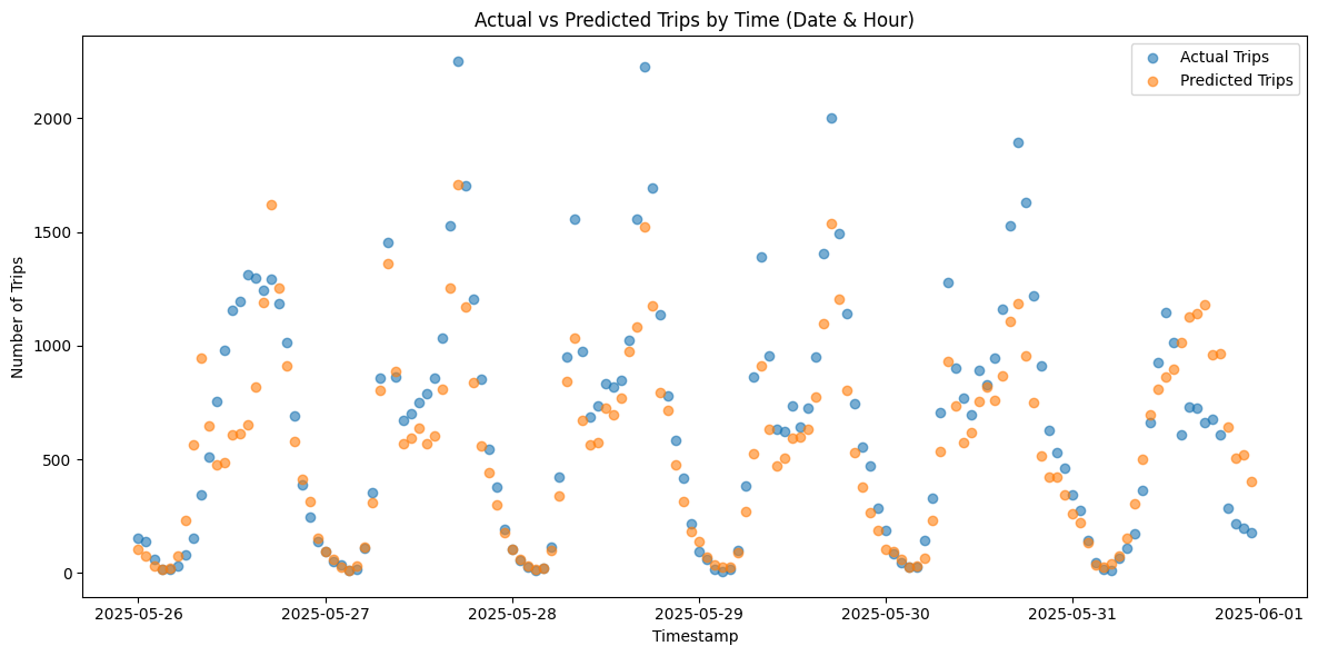
Applying this tuned regressor to the 6-day test set:
- Test MAE: 184.76 trips/hour
- Test RMSE: insert RMSE
7. Next Steps & Takeaways
- Feature Enrichment: Merge weather and special-event data for further accuracy gains.
- Advanced Methods: Explore hybrid ARIMA + ML stacks or temporal Transformers for long-range dependencies.
- Operationalization: Wrap the final model in a Flask API (or Docker container) for real-time demand queries.
Through this iterative process—from a basic linear fit to automated model‐racing and careful hyperparameter tuning—I achieved a robust demand‐forecasting pipeline that reduced MAE by ~30% compared to the baseline. The final model (Radius Neighbors with distance weighting) delivers reliable, fine‐grained predictions that Blue Bikes could integrate into their rebalancing and maintenance schedules.
Key Features
- Natural language understanding
- Context-aware responses
- Multi-language support
- Integration with various platforms
- Continuous learning capabilities